Fractal geometry
Fractal geometry is an opposite concept to classical or Euclidean geometry in that it deals with structures that have complexity at all scales, unlike Euclidean geometry where shapes like points, lines, and planes have well-defined and deterministic properties, such as finite area or volume. One of the most famous fractals is the coast of Britain. Unlike regular patterns like triangle, rectangel or circle, the length of a coastline can vary dramatically depending on the scale at which it is measured. (see Introduction for details).
What a fractal looks like?
Before the notion of fractal formally discovered in nature or built environment, humans had already been trying to create patterns and structures that exhibited complexity or had infinite length. The first group of people to show great interest in these complex patterns were mathematicians.
Cantor set
The concept of the Cantor set was introduced by the German-Russian mathematician Georg Cantor in the late 19th century. It is constructed by starting with a line segment (the largest interval), and then repeatedly dividing each remaining segment into three equal parts, removing the middle third each time. Cantor was deeply interested in the nature of infinity and wanted to understand different types of infinite sets. At the time, it was widely believed that all infinities were the same size, but Cantor showed that there are different sizes of infinity. The Cantor set, while uncountably infinite, has a counterintuitive property: it contains infinitely many points, yet its total length (in the traditional sense) is zero.
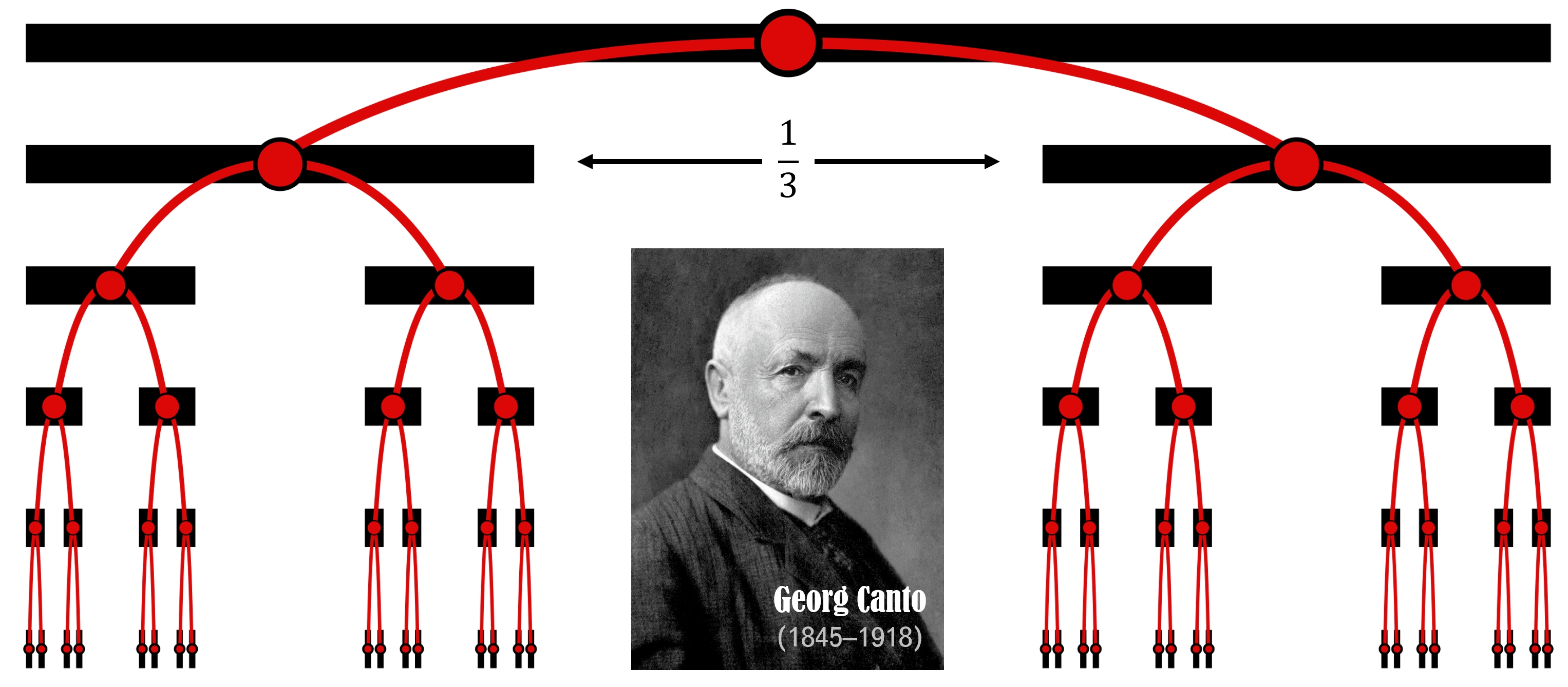
Similar to the coastline of Britain, the Cantor set shows infinite detail, making its total length unmeasurable in the traditional sense. The infinite complexity of the Cantor set arises from the process of repeated iterations—each step involves removing the middle third of each remaining segment. With each iteration, the set becomes more intricate, but crucially, the pattern self-repeats at every scale.
Koch curve
Koch curve is also a famous fractal but a 2D-shape. The Koch curve was invented by the Swedish mathematician Helge von Koch in 1904. Begin with a single straight line, it is divided into three parts and the middle part is replaced with two equivalent segments. Finally the process will lead to four new segments in each iteration.
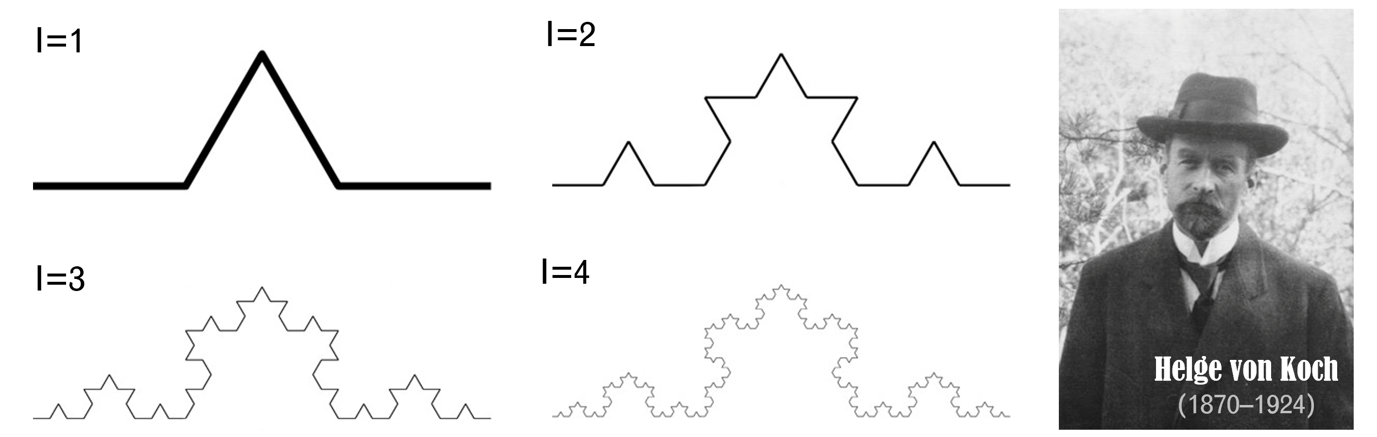
Different from the Cantor set, the Koch curve is closer to real-world features because it is continuous, whereas the Cantor set is discrete. The length of Koch curve is somehow infinite as long as it iterates for inifinite times. To construct the complex shape, you can see every new part is actually exactly the same pattern as the old one. This comes the first property of a fractal, that is the self-similarity.
Sierpiński triangle
Sierpiński triangle is conceived by Polish Mathamatician Wacław Sierpiński in 1915. It is considered to be more complex than both the Cantor set and Koch curve as it is based on a triangle.
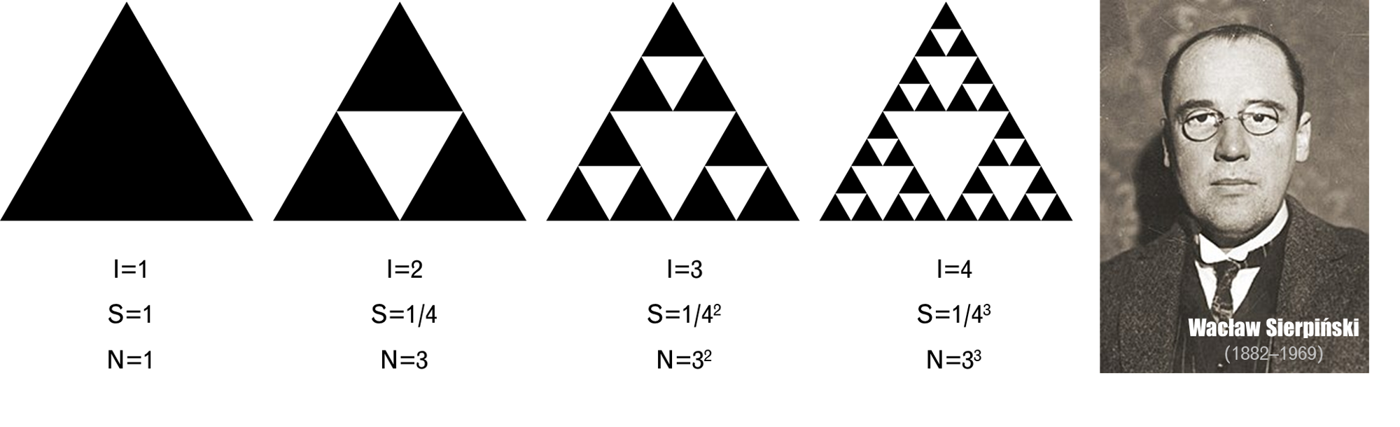
Every iteration it will divide itself into 4 exactly equal parts and remove the middle one. Thus, the Sierpiński triangle also shows strong self-similarity. (I denotes the times of iterations, S reprents the scale compared to the largest, and N means the numbers of details.)
What is a fractal?
In mathematics, a fractal is a geometric shape containing detailed structure at arbitrarily small scales (From Wikipedia). In other words, fractals exhibit self-similarity at each different scale. Across levels of scale, they all show a very complex pattern and details, much like the three patterns I mentioned above.
Exact self-similarity
Exact self-similarity means all patterns are identical at all scales, such as the Cantor set, Koch curve and Sierpiński triangle. And the most intersting thing is about how they scale. According to the exact self-similarity, the number of details will be exponentially increasing with the scale going down. Let’s draw a scatter plot for the three patterns.
You can see the scatter plot shows very strong long-tail characteristics. In other words, there are far more small details than large ones. It is kind of unclear to see the difference between the three distribution. But if we put them in log-log plot, they are three straight lines.
The long-tail distribution can be well described by a power law, where the frequency and the scale of a pattern are inversely proportional. The power law equation can be written as:
\[P(x) \propto x^{-\alpha}\]